The “Vlookup function” combined with the IF function would have to be some of the most used functions in all my Excel spreadsheets. The combination of these functions allows me to “look up” pieces of information from a list and perform some comparative analysis on my data. Very powerful stuff when you get the hang of it.
The Vlookup function does pretty much what its name suggests. It looks up a value in a vertical listing of data (hence the V in Vlookup) and returns information based on whether it finds the value or not.
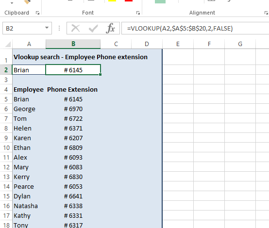
To give an example of how you can use the Vlookup function, lets say you want to look up an employee’s phone extension using their first name. See the image of our example spreadsheet below. Cell A2 is our input box (where we type our employee names) and cell B2 shows the result of our Vlookup function (employee phone number in this case).

Vlookup Function example
Vlookup Function
=VLOOKUP(lookup_value,table_array,col_index_num,range_lookup)1. lookup_value (required)
2. table_array (required)
3. col_index_num (required)
3. range_lookup (optional)
To use the Vlookup function in your spreadsheets, you will need 4 pieces of information.
- lookup_value
- table_array
- col_index_num
- range_lookup
At first, this function may seem very intimidating as the information it requires and the terminology used are not that simple to understand. But like most things, once you actually understand what the terms are and the pieces of information it requires, it is really quite simple to use and may end up being one of your most favourite functions to use in Excel (it is one of ours !!).
Let’s look now at the pieces of information we need for this function:
1. Lookup_value – This is quite straight forward and is the actual value that you are using the search to look for data in your list. In our example spreadsheet above, the lookup_value will be our employees’ name. The value in cell A2 in our example.
2. Table_array – This is the list of data (or range) that we will look in to find our lookup_value. In our example, this is the range of cells from A5 to B20 that contains all our employees names and their phone numbers. This data can be on our existing worksheet, as in our example, or another worksheet within your workbook. When defining a table_array there are a couple of rules and caveats that you must remember – these are shown in the following highlighted box.
Table_array
There are a couple of rules and caveats to remember with using the table_array.
Rules & CaveatsRule 1 – The Vlookup function works by looking up values in the leftmost column and finds a value in a column to the right of the first column.Rule 2 – The leftmost column of your table_array MUST contain the values you are looking up. In other words, in our example, the employee names must be listed in the first column of our table_array. I can not have the employee phone numbers in column A and names in column B when I am using the employees name as the lookup_value.Rule 3 – You should not have duplicate values in the leftmost column of your table_array. The Vlookup function only ever finds the very first instance of your lookup_value and ignores any that may exist after the first one.Rule 4 – When defining the range for your table_array, you want to make sure you use Absolute Cell References (“$” signs) so your range doesn’t automatically change if you copy this formula to another cell. In our example, the absolute cell reference we will use is $A$5:$B$20.
3. Col_index_num – This is the number of the column in your list of lookup data (table_array) that has the information you are wanting to bring back. In our example, we want to find the employees phone number and that is located in column 2 of our table_array.
4. Range-lookup – This defines how close a match you need between the lookup_value (employee name) and the values in the leftmost column on our table_array. You enter either “TRUE” or “FALSE” for this component of the function.
Range_lookup
1. FALSE – we want the vlookup function to find an EXACT match of the value we are looking up
2. TRUE – we want the vlookup function to find the closest match it can to our lookup value
Ok, so to complete the formula in our example using the vlookup function. The formula that we enter into cell B2 is:=vlookup(A2,$A$5:$B$20,2,false)that is – lookup up the value we enter into A2, in the range A5 to B20 and if you find an exact match bring back the value you find in the second column.
Please Share
If you have found value from this article or know someone who may be able to benefit from it, please feel free to share it with your friends and spread the word on Facebook, Twitter or Linkedin.


